Data Preprocessing
Notice: You don’t have to read this section for the contest
In this part, I will walk you through details of our data and introduce some data preprocessing procedures. I hope you could get a clear understanding of our data and are able to generate you own training dataset after this session.
Basically, we will use rat in vivo liver differential gene expression data as training data and use the corresponding pathology terms as labels. All these data can be extracted from TG-GATEs database. For your quickly understanding , imagine our training data as a matrix whose rows represent samples and columns represent features. In more details, each sample(row) represents differential gene expression levels in liver for a rat at certain time point and certain drug dose level. And each feature(column) represents expression level of a certain gene across different samples. Each sample has a pathological record for each pathology from TG-GATEs.
Gene expression data
Before we go further, let’s first introduce what is gene expression data. Gene is the basic physical and functional unit of heredity among all the species. Slight difference between genes decide individual’s unique physical features. Gene controls the traits or phenotypes of species by transcription and translation to RNAs and proteins. The expression level of transcription and translation can be detected by microarrays or next generation sequencing techniques(NGS), which is called gene expression data.
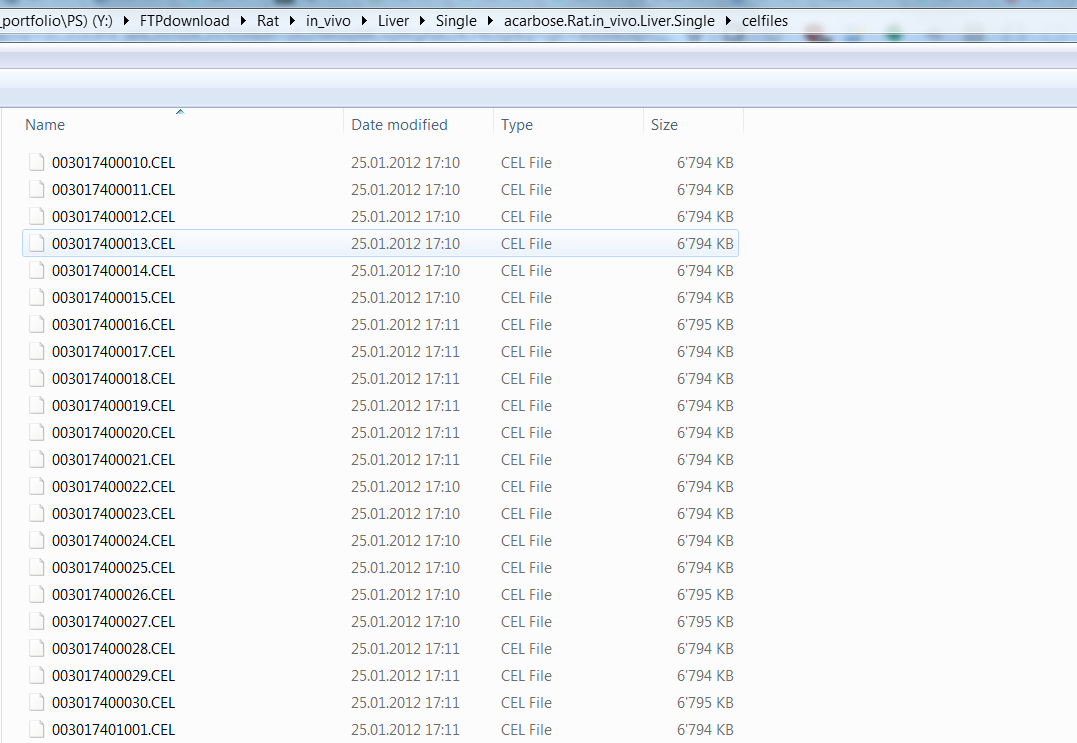
The gene expression levels in rat in vivo liver in TG-GATEs are measured by microarrays. So the results are stored in .CEL file format and all the CEL data pass the quality control QC
Then let’s get a intuitive understanding of gene expression data from rat in vivo liver that administered acarbose in single-dose experiment(See below what is single-dose experiment in TG-GATEs). In the folder of “TG-GATEs/rat/in_vivo/Liver/Single/acarbose.Rat.in_vivo.Liver.Single”, there is a folder called “celfiles” containing CEL files for each specific drug administered experiment. Another Attribute.csv file in this folder includes metadata for each CEL file in “celfiles” directory.

For example, the second row in Attribute.csv file have a attribute “BARCODE” with value “3017401004”
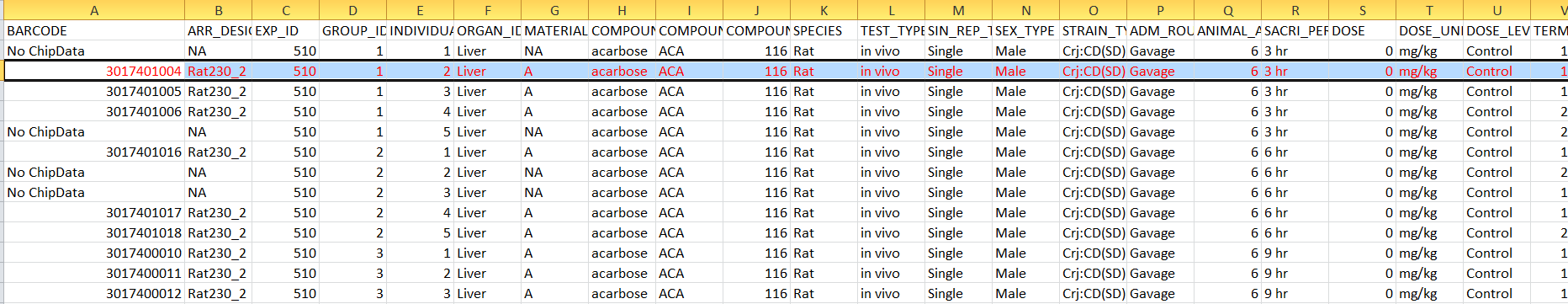
This means this row is meatadata for “003017401004.CEL” in “celfiles” folder.
The attributes “ORGAN”, “COMPOMD_NAME”,“SPECIES”,“TEST_TYPE”,“SIN_REP_TYPE”,“SACRI_PERIOD” and “DOSE_level” in second row of attributes file tell us “003017401004.CEL” containing the gene expression data of liver for rat administered acarbose, which was measured at 3 hour with dose level “control”. Notice for each experimental condition,there are several samples(i.e. Several CELfiles) to increase statistical power.
To obtain gene expression data, we load all the CEL data in this folder and preprocess them with R packages “affy”. This is necessary and reasons for this are explained in This paper
- Read all the CEL files from acarbose administered experiment by function “ReadAffy” to “AffyBatch” object
library(affy)
cell_dir="../TGGATEs_tutorial_secrete/acarbose.Rat.in_vivo.Liver.Single"
fns=list.celfiles(path=paste(cell_dir,"celfiles",sep = "/"),full.names=TRUE)
data=ReadAffy(filenames = fns)- Then we can use function “rma” in “affy” package to preprocess our data by following steps:
- Background correction
- Normalization
- Computation of expression data
Function “rma”" will transfer our “AffyBatch” object into “ExpressionSet” object. “ExpressionSet” object is a class frequently used in genomics to manage high-throughput assays and experimental meatadata.
eset=rma(data,normalize = TRUE)## Background correcting
## Normalizing
## Calculating Expressionhead(exprs(eset))## 003017400010.CEL 003017400011.CEL 003017400012.CEL
## 1367452_at 9.710680 9.821241 9.729149
## 1367453_at 9.067860 9.043074 9.235215
## 1367454_at 9.550044 9.606659 9.698128
## 1367455_at 10.553506 10.507285 10.594691
## 1367456_at 11.309212 11.347825 11.315577
## 1367457_at 8.360367 8.366649 8.510971
## 003017400013.CEL 003017400014.CEL 003017400015.CEL
## 1367452_at 9.815303 9.875462 9.608883
## 1367453_at 9.038412 9.138011 9.121376
## 1367454_at 9.619881 9.695400 9.504571
## 1367455_at 10.574645 10.607804 10.556159
## 1367456_at 11.251396 11.331002 11.308642
## 1367457_at 8.462920 8.516944 8.388226
## 003017400016.CEL 003017400017.CEL 003017400018.CEL
## 1367452_at 9.724402 9.817019 9.623560
## 1367453_at 9.070919 9.017824 9.073013
## 1367454_at 9.680938 9.648683 9.553031
## 1367455_at 10.526525 10.399546 10.481923
## 1367456_at 11.314574 11.206302 11.409712
## 1367457_at 8.381121 8.488152 8.336819
## 003017400019.CEL 003017400020.CEL 003017400021.CEL
## 1367452_at 9.748710 9.891357 9.718400
## 1367453_at 8.984381 9.094326 9.088472
## 1367454_at 9.543775 9.412876 9.551197
## 1367455_at 10.429839 10.292437 10.356549
## 1367456_at 11.391975 11.252916 11.379758
## 1367457_at 8.336397 8.478398 8.335831
## 003017400022.CEL 003017400023.CEL 003017400024.CEL
## 1367452_at 9.727142 9.701745 9.709448
## 1367453_at 9.062464 8.977847 8.976962
## 1367454_at 9.351506 9.365923 9.445604
## 1367455_at 10.280625 10.450370 10.451998
## 1367456_at 11.079971 11.190103 11.207608
## 1367457_at 8.025818 8.374099 8.414981
## 003017400025.CEL 003017400026.CEL 003017400027.CEL
## 1367452_at 9.733389 9.652379 9.632717
## 1367453_at 9.002082 8.910885 9.038838
## 1367454_at 9.236594 9.467579 9.267384
## 1367455_at 10.330430 10.284391 10.348205
## 1367456_at 11.098047 11.118901 11.141853
## 1367457_at 8.345019 8.383982 8.242447
## 003017400028.CEL 003017400029.CEL 003017400030.CEL
## 1367452_at 9.814365 9.727001 9.727374
## 1367453_at 9.111133 8.982413 8.987644
## 1367454_at 9.293652 9.322218 9.347107
## 1367455_at 10.284320 10.350225 10.469496
## 1367456_at 11.275095 11.192766 11.338031
## 1367457_at 8.384063 8.331452 8.371683
## 003017401001.CEL 003017401002.CEL 003017401004.CEL
## 1367452_at 9.718375 9.782471 9.623173
## 1367453_at 8.945542 9.096682 9.000747
## 1367454_at 9.318388 9.383579 9.423432
## 1367455_at 10.439494 10.347890 10.625569
## 1367456_at 11.219220 11.385027 11.209722
## 1367457_at 8.370650 8.384117 8.460935
## 003017401005.CEL 003017401006.CEL 003017401007.CEL
## 1367452_at 9.583269 9.560896 9.530430
## 1367453_at 9.159080 9.065309 8.995264
## 1367454_at 9.292879 9.614397 9.583177
## 1367455_at 10.315748 10.668048 10.449376
## 1367456_at 11.134747 11.294581 11.167560
## 1367457_at 8.378980 8.362393 8.344895
## 003017401008.CEL 003017401009.CEL 003017401010.CEL
## 1367452_at 9.499991 9.612328 9.559172
## 1367453_at 9.006853 9.062042 9.057569
## 1367454_at 9.595885 9.431221 9.480295
## 1367455_at 10.543703 10.560476 10.557472
## 1367456_at 11.143142 11.228497 11.150741
## 1367457_at 8.381121 8.209521 8.409710
## 003017401011.CEL 003017401012.CEL 003017401013.CEL
## 1367452_at 9.566836 9.622645 9.574145
## 1367453_at 9.061715 8.879621 8.959905
## 1367454_at 9.480752 9.673828 9.484616
## 1367455_at 10.487039 10.745641 10.548618
## 1367456_at 11.207408 11.200128 11.141184
## 1367457_at 8.268765 8.515319 8.362838
## 003017401014.CEL 003017401015.CEL 003017401016.CEL
## 1367452_at 9.541026 9.621357 9.403145
## 1367453_at 9.123613 9.165200 8.782882
## 1367454_at 9.565737 9.411885 9.389433
## 1367455_at 10.533120 10.565633 10.321440
## 1367456_at 11.156299 11.204316 11.045789
## 1367457_at 8.398465 8.403353 8.209383
## 003017401017.CEL 003017401018.CEL 003017401019.CEL
## 1367452_at 9.487107 9.375530 9.453894
## 1367453_at 8.917921 8.927603 8.857794
## 1367454_at 9.529719 9.397964 9.463278
## 1367455_at 10.515769 10.244465 10.394566
## 1367456_at 11.153529 11.142325 11.042324
## 1367457_at 8.200696 8.317639 8.178311
## 003017401020.CEL 003017401021.CEL 003017401022.CEL
## 1367452_at 9.472529 9.442826 9.446881
## 1367453_at 8.822515 8.981781 8.875951
## 1367454_at 9.461396 9.491253 9.523311
## 1367455_at 10.333446 10.442049 10.513276
## 1367456_at 11.067492 11.119393 11.060740
## 1367457_at 8.209951 8.103366 8.261018
## 003017401023.CEL 003017401024.CEL 003017401025.CEL
## 1367452_at 9.450991 9.393279 9.350718
## 1367453_at 8.962875 8.915636 9.072396
## 1367454_at 9.401245 9.433988 9.418821
## 1367455_at 10.552136 10.503325 10.585526
## 1367456_at 11.166481 11.137850 11.243584
## 1367457_at 8.179018 8.269388 8.199147
## 003017401026.CEL 003017401027.CEL 003017402020.CEL
## 1367452_at 9.516306 9.471616 9.721508
## 1367453_at 8.819234 8.817361 8.982944
## 1367454_at 9.529164 9.393140 9.349881
## 1367455_at 10.536884 10.370577 10.231311
## 1367456_at 11.202182 11.027853 11.278662
## 1367457_at 8.052840 8.048279 8.205769“exprs” function returns expression data of our experiment. Columns refer to samples and rows refer to probeset in microarray.
- From “Attribute.tsv”" file, we can add “phenoData” to “ExpressionSet” to describe samples in the experiment
pheno=read.table(paste(cell_dir,"/Attribute.tsv",sep = ""),sep = "\t",header = TRUE,fileEncoding="latin1")
pheno=pheno[which(pheno[,"BARCODE"]!="No ChipData"),]
rownames(pheno)=paste("00",sub('^0+',"",pheno[,"BARCODE"]),".CEL",sep = "")
pheno=pheno[colnames(exprs(eset)),]
pData(eset) = pheno
head(pData(eset))
## BARCODE ARR_DESIGN EXP_ID GROUP_ID INDIVIDUAL_ID
## 003017400010.CEL 003017400010 Rat230_2 510 3 1
## 003017400011.CEL 003017400011 Rat230_2 510 3 2
## 003017400012.CEL 003017400012 Rat230_2 510 3 3
## 003017400013.CEL 003017400013 Rat230_2 510 7 1
## 003017400014.CEL 003017400014 Rat230_2 510 7 2
## 003017400015.CEL 003017400015 Rat230_2 510 7 3
## ORGAN_ID MATERIAL_ID COMPOUND_NAME COMPOUND.Abbr.
## 003017400010.CEL Liver A acarbose ACA
## 003017400011.CEL Liver A acarbose ACA
## 003017400012.CEL Liver A acarbose ACA
## 003017400013.CEL Liver A acarbose ACA
## 003017400014.CEL Liver A acarbose ACA
## 003017400015.CEL Liver A acarbose ACA
## COMPOUND_NO SPECIES TEST_TYPE SIN_REP_TYPE SEX_TYPE
## 003017400010.CEL 116 Rat in vivo Single Male
## 003017400011.CEL 116 Rat in vivo Single Male
## 003017400012.CEL 116 Rat in vivo Single Male
## 003017400013.CEL 116 Rat in vivo Single Male
## 003017400014.CEL 116 Rat in vivo Single Male
## 003017400015.CEL 116 Rat in vivo Single Male
## STRAIN_TYPE ADM_ROUTE_TYPE ANIMAL_AGE.week.
## 003017400010.CEL Crj:CD(SD)IGS Gavage 6
## 003017400011.CEL Crj:CD(SD)IGS Gavage 6
## 003017400012.CEL Crj:CD(SD)IGS Gavage 6
## 003017400013.CEL Crj:CD(SD)IGS Gavage 6
## 003017400014.CEL Crj:CD(SD)IGS Gavage 6
## 003017400015.CEL Crj:CD(SD)IGS Gavage 6
## SACRI_PERIOD DOSE DOSE_UNIT DOSE_LEVEL TERMINAL_BW.g.
## 003017400010.CEL 9 hr 0 mg/kg Control 195.5
## 003017400011.CEL 9 hr 0 mg/kg Control 199.3
## 003017400012.CEL 9 hr 0 mg/kg Control 192.8
## 003017400013.CEL 9 hr 100 mg/kg Low 192.5
## 003017400014.CEL 9 hr 100 mg/kg Low 194.8
## 003017400015.CEL 9 hr 100 mg/kg Low 198.5
## LIVER.g. KIDNEY_TOTAL.g. KIDNEY_R.g. KIDNEY_L.g.
## 003017400010.CEL 8.359 1.711 0.874 0.837
## 003017400011.CEL 8.442 2.000 0.976 1.024
## 003017400012.CEL 7.501 1.747 0.869 0.878
## 003017400013.CEL 8.158 1.743 0.884 0.859
## 003017400014.CEL 7.180 1.750 0.854 0.896
## 003017400015.CEL 8.378 1.932 0.946 0.986
## RBC.x10_4.ul. Hb.g.dL. Ht... MCV.fL. MCH.pg. MCHC...
## 003017400010.CEL 647 13.3 40.8 63.1 20.5 32.5
## 003017400011.CEL 597 12.6 39.2 65.7 21.2 32.2
## 003017400012.CEL 625 13.0 39.9 63.8 20.8 32.6
## 003017400013.CEL 647 13.3 41.0 63.4 20.5 32.3
## 003017400014.CEL 657 12.7 39.3 59.8 19.4 32.4
## 003017400015.CEL 611 13.2 41.6 68.1 21.7 31.8
## Ret... Plat.x10_4.uL. WBC.x10_2.uL. Neu... Eos... Bas...
## 003017400010.CEL 7.1 136.4 98.0 18 1 0
## 003017400011.CEL 8.8 122.2 92.5 16 1 0
## 003017400012.CEL 8.9 100.4 81.8 14 0 0
## 003017400013.CEL 8.0 127.6 86.4 12 1 0
## 003017400014.CEL 8.0 111.2 68.6 22 1 0
## 003017400015.CEL 9.4 134.8 67.6 25 1 0
## Mono... Lym... PT.s. APTT.s. Fbg.mg.dL. ALP.IU.L.
## 003017400010.CEL 2 78 13.9 16.8 307 1358
## 003017400011.CEL 1 81 13.4 16.5 287 1889
## 003017400012.CEL 2 82 13.8 16.0 276 1373
## 003017400013.CEL 3 83 13.4 19.2 292 1478
## 003017400014.CEL 3 74 13.4 16.8 296 1195
## 003017400015.CEL 3 71 13.5 16.7 278 1309
## TC.mg.dL. TG.mg.dL. PL.mg.dL. TBIL.mg.dL. DBIL.mg.dL.
## 003017400010.CEL 76 58 134 0.06 0.01
## 003017400011.CEL 80 100 144 0.06 0.01
## 003017400012.CEL 61 42 114 0.06 0.01
## 003017400013.CEL 71 45 130 0.06 0.00
## 003017400014.CEL 89 99 143 0.05 0.00
## 003017400015.CEL 78 49 148 0.06 0.00
## GLC.mg.dL. BUN.mg.dL. CRE.mg.dL. Na.meq.L. K.meq.L.
## 003017400010.CEL 183 9 0.2 140 3.6
## 003017400011.CEL 199 7 0.2 140 4.1
## 003017400012.CEL 162 8 0.2 140 4.1
## 003017400013.CEL 179 7 0.2 139 3.8
## 003017400014.CEL 176 8 0.2 141 4.3
## 003017400015.CEL 169 8 0.2 142 3.7
## Cl.meq.L. Ca.mg.dL. IP.mg.dL. TP.g.dL. RALB.g.dL. A.G
## 003017400010.CEL 103 10.3 10.0 5.2 2.5 0.9
## 003017400011.CEL 104 10.5 9.3 5.0 2.4 0.9
## 003017400012.CEL 104 10.4 10.3 5.1 2.4 0.9
## 003017400013.CEL 103 10.5 9.3 5.3 2.5 0.9
## 003017400014.CEL 106 10.3 9.9 5.2 2.5 0.9
## 003017400015.CEL 105 10.5 9.8 5.5 2.6 0.9
## AST.IU.L. ALT.IU.L. LDH.IU.L. GTP.IU.L. DNA... LDH...
## 003017400010.CEL 72 40 57 2 NA NA
## 003017400011.CEL 72 34 78 1 NA NA
## 003017400012.CEL 64 31 59 1 NA NA
## 003017400013.CEL 71 40 60 1 NA NA
## 003017400014.CEL 69 33 69 1 NA NA
## 003017400015.CEL 67 39 63 1 NA NA- Annotate probesets of microarray to gene names by ribiosAnnotation to describe features in the experiment. Since each gene is usually represented by more than on probeset, we use ribiosUtils to further preprocess data to get unique gene names for our data .
library(ribiosAnnotation)
library(ribiosUtils)
geneName=annotateProbesets(featureNames(eset), orthologue = TRUE)
fData(eset) <- geneName
eset_rmNA=eset[!is.na(fData(eset)[,"GeneID"]),]
index_uniqueProbe=isMaxStatRow(exprs(eset_rmNA),keys = fData(eset_rmNA)[,"GeneSymbol"])
eset=eset_rmNA[index_uniqueProbe,]- After we get expression data, we remove gene with expression level less than 6 as these data are unreliable
eset <- eset[apply(exprs(eset), 1, max, na.rm=TRUE)>6,]Diffrential gene expression data
But here we use differential gene expression data other than gene expression data mainly because of batch effect as TG-GATEs is a long period(10 years) project conducted by various institutes and companies.
Differential gene expression data means quantitative changes of gene expression level between different experimental groups. Here we calculate differential gene expression for each experimental condition compared with control experimental condition.
The method we used to calculate differential gene expression data is called limma,which is a R package that fit a linear model to the expression data for each gene. By elaborate design matrix and contrast matrix, we can get various statistics from limma to (e.g. log folder changes and moderated t-statistics) describe differential gene expression data.
Below is the code we used to obtain differential gene expression data for one drug.
library(limma)
# the function used to calculate diffrential gene expression data
# regard experiment with dose level "control" and earliest time point as control group

limmaTG<-function(eset_timei_contrast,filename){
   f=factor(eset_timei_contrast$DOSE_LEVEL)
   # get dose information
   uni_levels=unique(f)
   level=uni_levels[-(which(uni_levels=="Control"))]
   # get csww information,  csww contains compound type, species, in vitro/vivo and organism information
   csww=tail(unlist(strsplit(filename,"/")),n=1)
   #get time information
   timepoint=unique(pData(eset_timei_contrast)$SACRI_PERIOD)
   # get sample name
   sample_name=paste(csww,timepoint,level,sep = "/")
   design=model.matrix(~+f)
   fit=lmFit(eset_timei_contrast,design)
   fit=eBayes(fit)
   nenv=new.env()
   #add logFC data as differential gene  experssion data
   fit_topTable <- topTable(fit,coef = 2,number = nrow(fit$genes))
   fit_exprs=matrix(fit_topTable$logFC)
   #rownames(fit_exprs)=rownames(fit$genes)  ## errors here ,fuck
   rownames(fit_exprs)=fit_topTable$GeneSymbol  ## when using some function, you'd better understand its
                                             ## function exactly
   colnames(fit_exprs)=sample_name
   #plot(fit_exprs,fit_topTable$logFC)
   assign("exprs",fit_exprs,nenv)

   fit_eset=ExpressionSet(assayData = nenv)
   fit_pheno=data.frame(time=timepoint,dose=level,csww=csww)
   rownames(fit_pheno)=colnames(fit_exprs)
   pData(fit_eset)=fit_pheno

   fData(fit_eset)=fit$genes
   return(fit_eset)

}

# obtain all the experimental time points
time_points=unique(pData(eset)$SACRI_PERIOD)
esets=list()
# loop used to calculate diffrential gene expression data for all the experimental groups compared with corrsponding control gruops
for (i in 1:length(time_points)) {
   eset_timei=eset[,which(pData(eset)$SACRI_PERIOD==time_points[i])]
   dose_levels=unique(pData(eset_timei)$DOSE_LEVEL)
   dose_levels=dose_levels[-which(dose_levels=="Control")]
   eset_timei_contrasts=list()
   for (ii in 1:length(dose_levels)) {
     eset_timei_contrasts[[ii]]=eset_timei[,c(which(eset_timei$DOSE_LEVEL=="Control"),which(eset_timei$DOSE_LEVEL==dose_levels[ii]))]
   }
   esets[[i]]=lapply(eset_timei_contrasts, limmaTG,filename=cell_dir)
}

 #combine all diffrential gene expression data of this certain compound into one
 compound_esets=list()
 index=1
 for (i in 1:length(esets)) {
   for (j in 1:length(esets[[i]])) {
     compound_esets[[index]]=esets[[i]][[j]]
     index=index+1
   }
 }
 fenv=new.env()

 compound_common_features=rownames(compound_esets[[1]])
 for (i  in 2:length(compound_esets) ) {
   compound_common_features=intersect(compound_common_features,rownames(compound_esets[[i]]))
 }

 for (i in 1:length(compound_esets)) {
   compound_esets[[i]]=compound_esets[[i]][compound_common_features,]
 }

 compound_exprs=sapply(compound_esets,exprs)
 rownames(compound_exprs)=rownames(compound_esets[[1]])
 colnames(compound_exprs)=sapply(compound_esets, function(x){colnames(exprs(x))})
 assign("exprs",compound_exprs,fenv)


 compound_final_eset=ExpressionSet(assayData = fenv)
 compound_pheno=lapply(compound_esets, pData)
 compound_pheno=do.call("rbind",compound_pheno)
 pData(compound_final_eset)=compound_pheno

 fData(compound_final_eset)=fData(compound_esets[[1]])
 saveRDS(compound_final_eset,file = paste(cell_dir,".rds",sep = ""))
From above, we get a “ExpressionSet” object storing differential gene expression data from a specific drug experiment. We write it into a “.rds” R data for further data combination
drug_exprs=exprs(compound_final_eset)
head(drug_exprs)
## acarbose.Rat.in_vivo.Liver.Single/9 hr/Low
## EML1 -1.0641666
## KLHL25 0.8963165
## FRG1HP -0.7605153
## SIGLEC6 -0.9695392
## ACOX2 -0.8439054
## SERPINB1 -0.5448026
## acarbose.Rat.in_vivo.Liver.Single/9 hr/Middle
## EML1 -1.0875654
## KLHL25 0.2866352
## FRG1HP -0.7672887
## SIGLEC6 -0.2913878
## ACOX2 -0.3945244
## SERPINB1 -0.1584559
## acarbose.Rat.in_vivo.Liver.Single/9 hr/High
## EML1 -0.26436814
## KLHL25 -0.11820882
## FRG1HP -0.80605145
## SIGLEC6 -0.93826882
## ACOX2 -0.57276976
## SERPINB1 -0.08946052
## acarbose.Rat.in_vivo.Liver.Single/24 hr/Low
## EML1 -0.027796717
## KLHL25 0.011789954
## FRG1HP -0.002698597
## SIGLEC6 0.190932121
## ACOX2 -0.038851037
## SERPINB1 0.305954269
## acarbose.Rat.in_vivo.Liver.Single/24 hr/Middle
## EML1 0.1914574
## KLHL25 -0.3949797
## FRG1HP 0.1913012
## SIGLEC6 0.2146495
## ACOX2 -0.2757300
## SERPINB1 0.2151618
## acarbose.Rat.in_vivo.Liver.Single/24 hr/High
## EML1 0.14735667
## KLHL25 -0.11686737
## FRG1HP 0.08786183
## SIGLEC6 0.19145517
## ACOX2 -0.11554888
## SERPINB1 0.25695981
## acarbose.Rat.in_vivo.Liver.Single/3 hr/Low
## EML1 -0.55787683
## KLHL25 0.08002887
## FRG1HP 0.29394250
## SIGLEC6 0.18472591
## ACOX2 0.25228829
## SERPINB1 0.23205854
## acarbose.Rat.in_vivo.Liver.Single/3 hr/Middle
## EML1 -0.61668202
## KLHL25 -0.23188214
## FRG1HP -0.12422623
## SIGLEC6 -0.02300787
## ACOX2 0.24001352
## SERPINB1 0.24890612
## acarbose.Rat.in_vivo.Liver.Single/3 hr/High
## EML1 0.1165509
## KLHL25 -0.2846511
## FRG1HP 0.1506972
## SIGLEC6 0.7458388
## ACOX2 0.4316805
## SERPINB1 -0.0454757
## acarbose.Rat.in_vivo.Liver.Single/6 hr/Low
## EML1 0.05201009
## KLHL25 0.22859480
## FRG1HP -0.29416223
## SIGLEC6 -0.15900132
## ACOX2 0.24934787
## SERPINB1 0.05049851
## acarbose.Rat.in_vivo.Liver.Single/6 hr/Middle
## EML1 0.16226183
## KLHL25 0.32564287
## FRG1HP 0.02491137
## SIGLEC6 -0.51976819
## ACOX2 0.41886287
## SERPINB1 0.16531870
## acarbose.Rat.in_vivo.Liver.Single/6 hr/High
## EML1 0.07240130
## KLHL25 0.04466170
## FRG1HP -0.22538618
## SIGLEC6 -1.08564083
## ACOX2 -0.09675233
## SERPINB1 0.30231961Experimental design in TG-GATEs
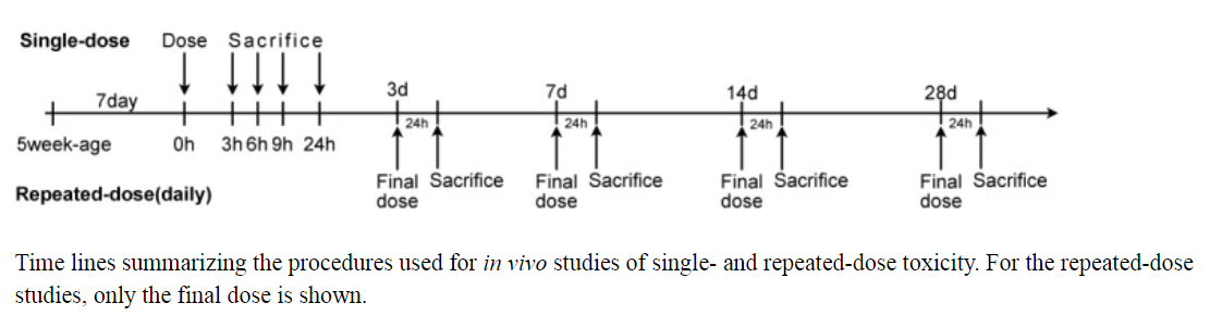
There are two types of studies to measure gene expression data from rat in vivo liver : single-dose study and repeat-dose study. " For single-dose experiments, groups of 20 animals were administered a compound and then five animals/time point were sacrificed at 3, 6, 9 or 24 h after administration. For repeated-dose experiments, groups of 20 animals received a single dose per day of a compound and five animals/time point were sacrificed at 4, 8, 15 or 29 days (i.e. 24 h after the respective final administration at 3, 7, 14 or 28 days )"
Data combination
In data combination step, we combine differential gene expression data(i.e. “.rds” data we stored in data preprocessing step) from different compounds in two types of studies. Besides, from pathology information in TG-GATEs, we extract pathology terms for corresponding samples. Please see the Easy Start section for final data format.
Copyright © 2018 F.Hoffmann-La Roche Ltd-All rights reserved.